
| 일 | 월 | 화 | 수 | 목 | 금 | 토 |
|---|---|---|---|---|---|---|
| 1 | 2 | 3 | 4 | 5 | 6 | 7 |
| 8 | 9 | 10 | 11 | 12 | 13 | 14 |
| 15 | 16 | 17 | 18 | 19 | 20 | 21 |
| 22 | 23 | 24 | 25 | 26 | 27 | 28 |
| 29 | 30 |
- 크롤링
- 플러터
- 자연어처리
- 선형대수학
- 인공지능
- 피플
- Regression
- 크롤러
- CV
- map
- 머신러닝
- Flutter
- filtering
- 코딩애플
- 42서울
- pytorch
- Computer Vision
- 선형회귀
- 모델
- 유데미
- 42경산
- RNN
- 파이썬
- 회귀
- 지정헌혈
- mnist
- 데이터분석
- 앱개발
- 딥러닝
- AI
- Today
- Total
David의 개발 이야기!
CNN을 활용한 MNIST 분류 모델 구현 본문
CNN 을 활용하여 MNIST 분류 모델을 구현해보자.
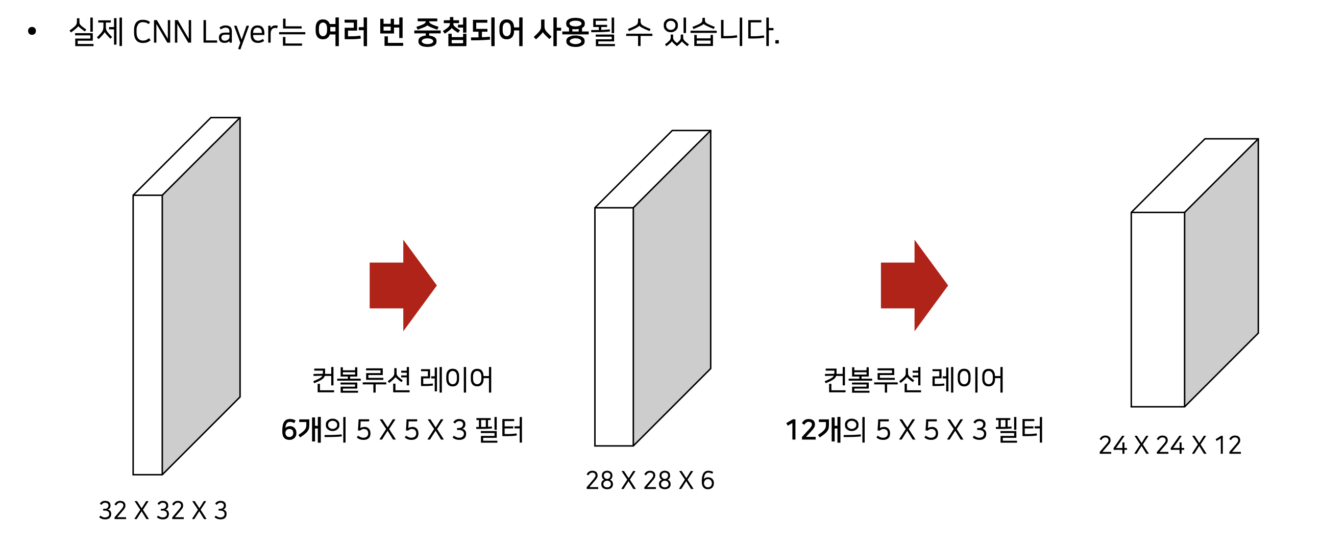
우선, CNN에 대한 개념 정리를 다시 보면,
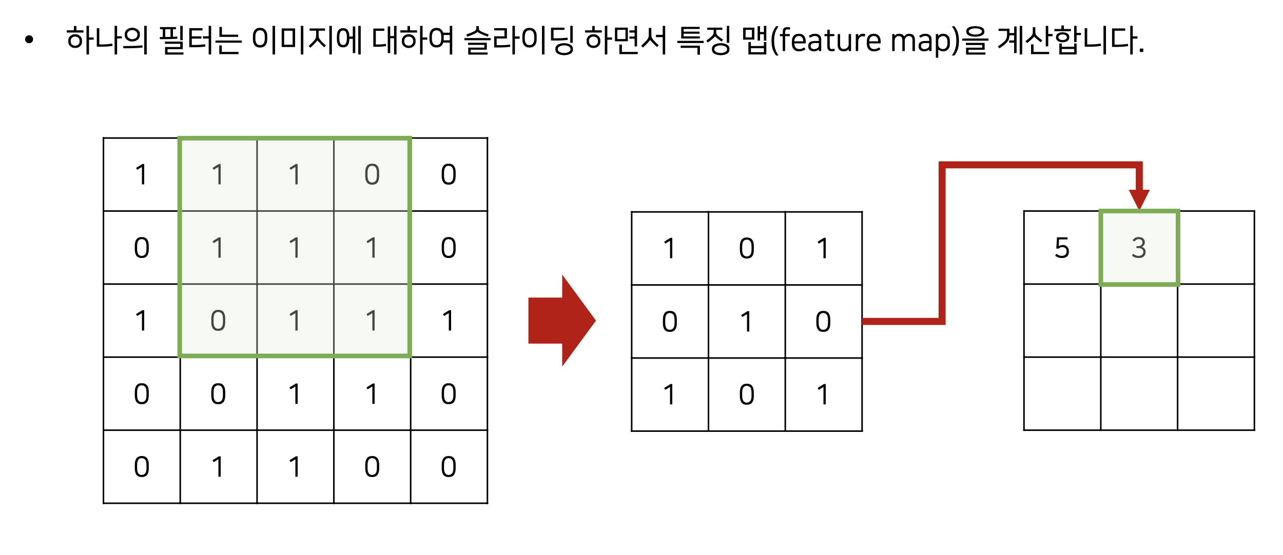
1. filter(==kernel) 개념
- 실제로 각 필터는, 특정한 (feature)를 인식하기 위한 목적으로 사용된다.
- 각 필터는 특징이 반영된 특징 맵(feature map)을 생성한다.
- 얕은 층에서는 local feature, 깊은 층에서는 global feature를 인식하는 경향이 있다.

2. Pooling 개념
합성곱 계층의 출력데이터를 입력으로 받아, 출력 데이터의 크기를 줄이거나, 특정 데이터를 강조하는 용도로 사용
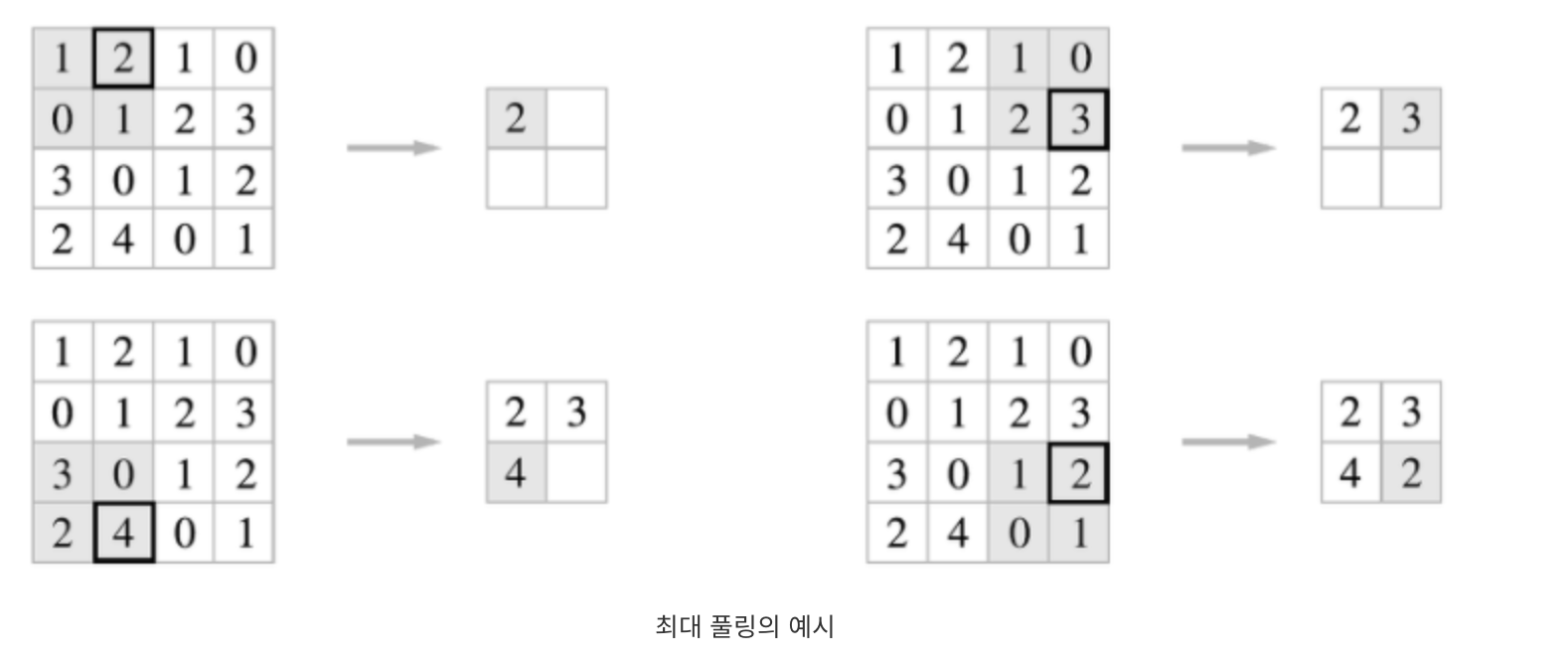
stride 가 2인 경우의 예시임.
3. Padding 개념
패딩이 필요한 이유
-> 이미지 데이터의 축소를 막기 위해(해상도를 유지하기 위해)
-> Edge pixel data(가장자리에 있는 데이터)를 충분히 활용하기 위해
4. CNN을 활용한 MNIST 분류 모델 구현
1. 필요한 라이브러리 불러오기
import torch
import torch.nn as nn
import torch.nn.functional as F
import torch.optim as optim

import torchvision
import torchvision.transforms as transforms

from matplotlib import pyplot as plt
import seaborn as sn
import pandas as pd
import numpy as np
import os

device = 'cuda'
2. 데이터세트 다운로드 및 불러오기
transform_train = transforms.Compose([
    transforms.ToTensor(),
])

transform_test = transforms.Compose([
    transforms.ToTensor(),
])

train_dataset = torchvision.datasets.MNIST(root='./data', train=True, download=True, transform=transform_train)
test_dataset = torchvision.datasets.MNIST(root='./data', train=False, download=True, transform=transform_test)

train_loader = torch.utils.data.DataLoader(train_dataset, batch_size=128, shuffle=True, num_workers=4)
test_loader = torch.utils.data.DataLoader(test_dataset, batch_size=100, shuffle=False, num_workers=4)
data augementation 등 사용할때, transform.Compose()안에 코드 추가
train_dataset, test_dataset 은, torchvision.datasets.MNIST에서 MNIST 데이터를 다운로드하고 불러옴
train_loader 는, 학습 데이터 셋을 로드하며, 배치 크기가 128로 설정되어 있음. 각 에폭마다, 데이터는 무작위로 섞여서 학습됨.
num_workers=4 이므로 4개의 프로세스를 사용하여 데이터 로드
test_loader 는 테스트 데이터셋을 로드하며, 배치크기가 100으로 설정되어 있음. 테스트 데이터 셋은 섞을 필요가 없어, shuffle=False로 되어 있음.
3. 학습(Training) 및 평가(Testing) 함수 정의
def train(net, epoch, optimizer, criterion, train_loader):
    print('[ Train epoch: %d ]' % epoch)
    net.train()
    train_loss = 0
    correct = 0
    total = 0
    for batch_idx, (inputs, targets) in enumerate(train_loader):
        inputs, targets = inputs.to(device), targets.to(device)
        optimizer.zero_grad()

        benign_outputs = net(inputs)
        loss = criterion(benign_outputs, targets)
        loss.backward()

        optimizer.step()
        train_loss += loss.item()
        _, predicted = benign_outputs.max(1)

        total += targets.size(0)
        correct += predicted.eq(targets).sum().item()

    print('Train accuarcy:', 100. * correct / total)
    print('Train average loss:', train_loss / total)
    return (100. * correct / total, train_loss / total)


def evaluate(net, epoch, file_name, data_loader, info):
    print('[ Evaluate epoch: %d ]' % epoch)
    print("Dataset:", info)

    net.eval() # Dropout을 적용하는 경우 필수임
    test_loss = 0
    correct = 0
    total = 0

    for batch_idx, (inputs, targets) in enumerate(data_loader):
        inputs, targets = inputs.to(device), targets.to(device)
        total += targets.size(0)

        outputs = net(inputs)
        test_loss += criterion(outputs, targets).item()

        _, predicted = outputs.max(1)
        correct += predicted.eq(targets).sum().item()

    print('Accuarcy:', 100. * correct / total)
    print('Average loss:', test_loss / total)
    return (100. * correct / total, test_loss / total)
[train 함수]
print('[ Train epoch: %d ]' % epoch): 현재 학습 에폭을 출력
net.train(): 신경망을 학습 모드로 설정. 이는 Dropout이나 Batch Normalization 같은 레이어가 다르게 동작하게끔 해줌
for batch_idx, (inputs, targets) in enumerate(train_loader):
inputs, targets = inputs.to(device), targets.to(device)
학습 데이터셋을 순회하기 위한 for 루프를 시작
input 과 target(정답 label)을 지정된 디바이스(CPU 또는 GPU)로 이동
optimizer.zero_grad():
이전의 gradient를 초기화 입력 데이터에 대해 신경망을 전방향으로 실행하여 출력
loss = criterion(benign_outputs, targets):
예측된 출력과 실제 타겟 사이의 손실을 계산
loss.backward():
gradient를 역전파
optimizer.step():
최적화 알고리즘을 사용해 신경망의 가중치를 업데이트
train_loss += loss.item()
- loss는 현재 배치(batch)에 대한 손실 값. item() 함수는 이 손실 값을 scalar 값으로 변환
- train_loss는 모든 배치에 대한 손실을 누적하기 위해 사용되며, train_loss에 현재 배치의 손실을 더함
_, predicted = benign_outputs.max(1)
- benign_outputs는 네트워크의 출력값. 여기서 max(1) 함수는 각 샘플에 대해 가장 높은 값을 가진 인덱스(즉, 가장 확률이 높은 클래스)를 반환.
- predicted에는 가장 높은 확률을 가진 클래스의 인덱스들이 저장.
- benign_outputs() 에서 반환되는 값은 두개의 텐서로, 첫번째 텐서는, 각 입력샘플에 대한 최대 출력값, 두번째 텐서는 해당 최대값의 인덱스. 이 인덱스가 결국 클래스 번호라고 볼 수 있음(뒤에거만 의미 있는 거임)
total += targets.size(0):
- targets.size(0)은 현재 배치의 샘플 개수를 반환
- total에 현재 배치의 샘플 수를 더해 전체 샘플의 수를 누적
correct += predicted.eq(targets).sum().item():
- predicted.eq(targets)는 predicted와 targets가 같은지 비교하여 Boolean 타입의 텐서를 반환
- sum()은 True 값들 (올바르게 예측된 샘플 수)을 합산
- item() 함수는 이 값을 scalar 값으로 변환
- 이렇게 계산된 올바르게 예측된 샘플 수를 correct에 누적
[evalutate 함수]
for batch_idx, (inputs, targets) in enumerate(data_loader):
데이터 로더에서 각 배치를 순차적으로 가져옴. batch_idx는 현재 배치의 인덱스 번호이며, inputs는 이미지 데이터 배치이고, targets는 해당 이미지 데이터의 정답 레이블 배치.
total += targets.size(0)
total 변수는 현재까지 처리한 샘플의 총 개수를 추적. targets.size(0)은 현재 배치의 샘플 수를 반환
outputs = net(inputs)
모델에 현재의 inputs 배치를 전달하여 예측 결과를 얻습니다
test_loss += criterion(outputs, targets).item()
모델의 출력(outputs)과 실제 레이블(targets)을 사용하여 손실을 계산하고, 이 손실 값을 test_loss에 누적
_, predicted = outputs.max(1)
모델의 출력에서 가장 높은 값을 가진 클래스의 인덱스를 얻음. 이 인덱스는 모델의 예측된 레이블. 여기서 _는 각 클래스의 최대 확률 값들을 무시하기 위해 사용
correct += predicted.eq(targets).sum().item()
예측된 레이블(predicted)과 실제 레이블(targets)이 일치하는지 확인. 일치하는 경우의 총 수를 correct에 누적
4. 혼동행렬(Confususion Matrix) 함수 정의
def get_confusion_matrix(net, num_classes, data_loader):
    confusion_matrix = torch.zeros(num_classes, num_classes)

    net.eval() # Dropout을 적용하는 경우 필수임

    for batch_idx, (inputs, targets) in enumerate(data_loader):
        inputs, targets = inputs.to(device), targets.to(device)

        outputs = net(inputs)
        _, predicted = outputs.max(1)

        for t, p in zip(targets.view(-1), predicted.view(-1)):
            confusion_matrix[t.long(), p.long()] += 1

    return confusion_matrix
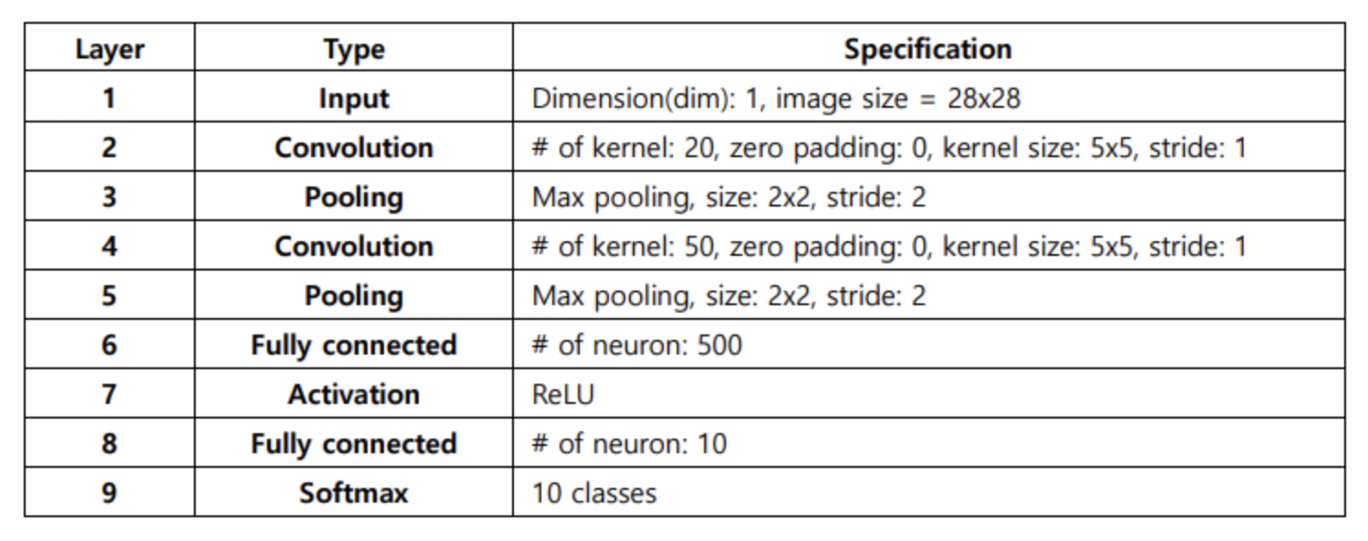
5. LeNet 모델 정의
class LeNet(nn.Module):
    # 실제로 가중치가 존재하는 레이어만 객체로 만들기
    def __init__(self):
        super(LeNet, self).__init__()
        # 여기에서 (1 x 28 x 28)
        # 입력 채널: 1, 출력 채널: 20 (커널 20개)
        self.conv1 = nn.Conv2d(in_channels=1, out_channels=20, kernel_size=5, stride=1, padding=0)
        # 여기에서 (20 x 24 x 24)
        # 풀링 이후에 (20 x 12 x 12)
        # 입력 채널: 20, 출력 채널: 50 (커널 50개)
        self.conv2 = nn.Conv2d(in_channels=20, out_channels=50, kernel_size=5, stride=1, padding=0)
        # 여기에서 (50 x 8 x 8)
        # 풀링 이후에 (50 x 4 x 4)
        self.fc1 = nn.Linear(50 * 4 * 4, 500)
        self.fc2 = nn.Linear(500, 10)

    def forward(self, x):
        x = F.max_pool2d(self.conv1(x), (2, 2))
        x = F.max_pool2d(self.conv2(x), (2, 2))
        x = x.view(-1, self.num_flat_features(x))
        x = F.relu(self.fc1(x))
        x = self.fc2(x)
        return x

    # 3차원의 컨볼루션 레이어를 flatten
    def num_flat_features(self, x):
        size = x.size()[1:] # 배치는 제외하고
        num_features = 1
        for s in size:
            num_features *= s
        return num_features
- forward 함수는, 신경망의 순방향 연산을 모두 계산하며, x가 주어지면, 출력까지 모든 계산이 여기서 수행된다.
- num_flat_features 함수는, 주어진 텐서의 모든 차원의 요소개수(feature)개수를 반환한다. 3D텐서를 1D텐서로 평면화할때 필요한 길이를 알아내기 위해 사용한다.
6. AlexNet 모델 정의

class LocalResponseNorm(nn.Module):
    def __init__(self, size, alpha = 1e-4, beta = 0.75, k = 1.0):
        super(LocalResponseNorm, self).__init__()
        self.size = size
        self.alpha = alpha
        self.beta = beta
        self.k = k

    def forward(self, input):
        return F.local_response_norm(input, self.size, self.alpha, self.beta, self.k)
class AlexNet(nn.Module):
def __init__(self):
super(AlexNet, self).__init__()
self.features = nn.Sequential(
# 여기에서 (1 x 28 x 28)
# 입력 채널: 1, 출력 채널: 96 (커널 96개)
nn.Conv2d(1, 96, kernel_size=5, stride=1, padding=2),
nn.ReLU(inplace=True),
LocalResponseNorm(size=5),
# 여기에서 (96 x 28 x 28)
nn.MaxPool2d(kernel_size=3, stride=2),
# 여기에서 (96 x 13 x 13)
# 입력 채널: 96, 출력 채널: 256 (커널 256개)
nn.Conv2d(96, 256, kernel_size=5, stride=1, padding=2),
nn.ReLU(inplace=True),
LocalResponseNorm(size=5),
# 여기에서 (256 x 13 x 13)
nn.MaxPool2d(kernel_size=3, stride=2),
# 여기에서 (256 x 6 x 6)
# 입력 채널: 256, 출력 채널: 384 (커널 384개)
nn.Conv2d(256, 384, kernel_size=3, stride=1, padding=1),
# 여기에서 (384 x 6 x 6)
nn.ReLU(inplace=True),
# 입력 채널: 384, 출력 채널: 384 (커널 384개)
nn.Conv2d(384, 384, kernel_size=3, stride=1, padding=1),
# 여기에서 (384 x 6 x 6)
nn.ReLU(inplace=True),
# 입력 채널: 384, 출력 채널: 384 (커널 384개)
nn.Conv2d(384, 384, kernel_size=3, stride=1, padding=1),
# 여기에서 (384 x 6 x 6)
nn.ReLU(inplace=True),
nn.MaxPool2d(kernel_size=3, stride=2),
# 여기에서 (384 x 2 x 2)
)
self.classifier = nn.Sequential(
nn.Linear(384 * 2 * 2, 2304),
nn.ReLU(inplace=True),
nn.Dropout(),
nn.Linear(2304, 10),
nn.Dropout(),
)
def forward(self, x):
x = self.features(x)
x = torch.flatten(x, 1)
x = self.classifier(x)
return x
7. LeNet 결과 분석
net = LeNet()
net = net.to(device)

epoch = 10
learning_rate = 0.01
file_name = "LeNet_MNIST.pt"

criterion = nn.CrossEntropyLoss()
optimizer = optim.SGD(net.parameters(), lr=learning_rate, momentum=0.9, weight_decay=0.0002)

train_result = []
test_result = []

train_result.append(evaluate(net, 0, file_name, train_loader, "Train"))
test_result.append(evaluate(net, 0, file_name, test_loader, "Test"))

for i in range(epoch):
    train(net, i, optimizer, criterion, train_loader)
    train_acc, train_loss = evaluate(net, i + 1, file_name, train_loader, "Train")
    test_acc, test_loss = evaluate(net, i + 1, file_name, test_loader, "Test")

    state = {
        'net': net.state_dict()
    }
    if not os.path.isdir('checkpoint'):
        os.mkdir('checkpoint')
    torch.save(state, './checkpoint/' + file_name)
    print('Model Saved!')

    train_result.append((train_acc, train_loss))
    test_result.append((test_acc, test_loss))
마지막 epoch 모델을 저장하는 코드 -> 가장 좋은 성능을 보이는 epoch 의 모델을 저장하게끔 수정 필요
accuracy 커브 시각화
# 정확도(accuracy) 커브 시각화
plt.plot([i for i in range(epoch + 1)], [i[0] for i in train_result])
plt.plot([i for i in range(epoch + 1)], [i[0] for i in test_result])
plt.xlabel("Epoch")
plt.ylabel("Accuracy")
plt.legend(["train", "test"])
plt.show()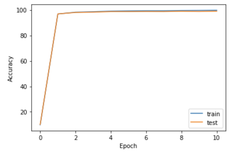
loss 커브 시각화
# 손실(loss) 커브 시각화
plt.plot([i for i in range(epoch + 1)], [i[1] for i in train_result])
plt.plot([i for i in range(epoch + 1)], [i[1] for i in test_result])
plt.xlabel("Epoch")
plt.ylabel("Loss")
plt.legend(["train", "test"])
plt.show()
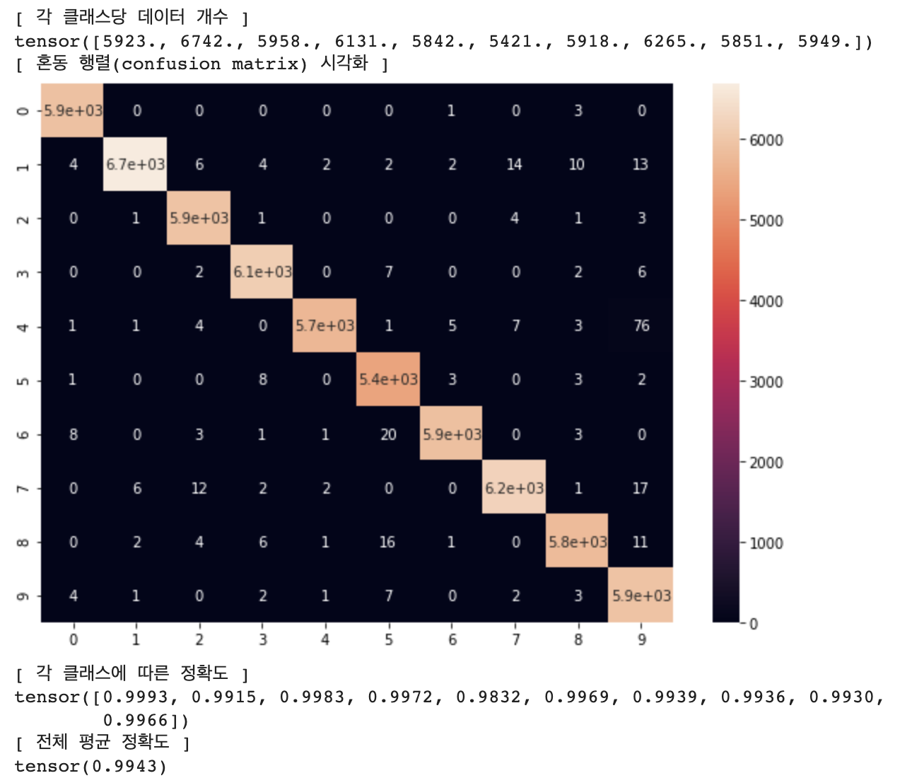
# 혼동 행렬(Confusion Matrix) 시각화 (학습 데이터셋)
net = LeNet()
net = net.to(device)

file_name = "./checkpoint/LeNet_MNIST.pt"
checkpoint = torch.load(file_name)
net.load_state_dict(checkpoint['net'])

confusion_matrix = get_confusion_matrix(net, 10, train_loader)
print("[ 각 클래스당 데이터 개수 ]")
print(confusion_matrix.sum(1))

print("[ 혼동 행렬(confusion matrix) 시각화 ]")
# 행(row)은 실제 레이블, 열(column)은 모델이 분류한 레이블
res = pd.DataFrame(confusion_matrix.numpy(), index = [i for i in range(10)], columns = [i for i in range(10)])
plt.figure(figsize = (10, 7))
sn.heatmap(res, annot=True)
plt.show()

print("[ 각 클래스에 따른 정확도 ]")
# (각 클래스마다 정답 개수 / 각 클래스마다 데이터의 개수)
print(confusion_matrix.diag() / confusion_matrix.sum(1))

print("[ 전체 평균 정확도 ]")
print(confusion_matrix.diag().sum() / confusion_matrix.sum())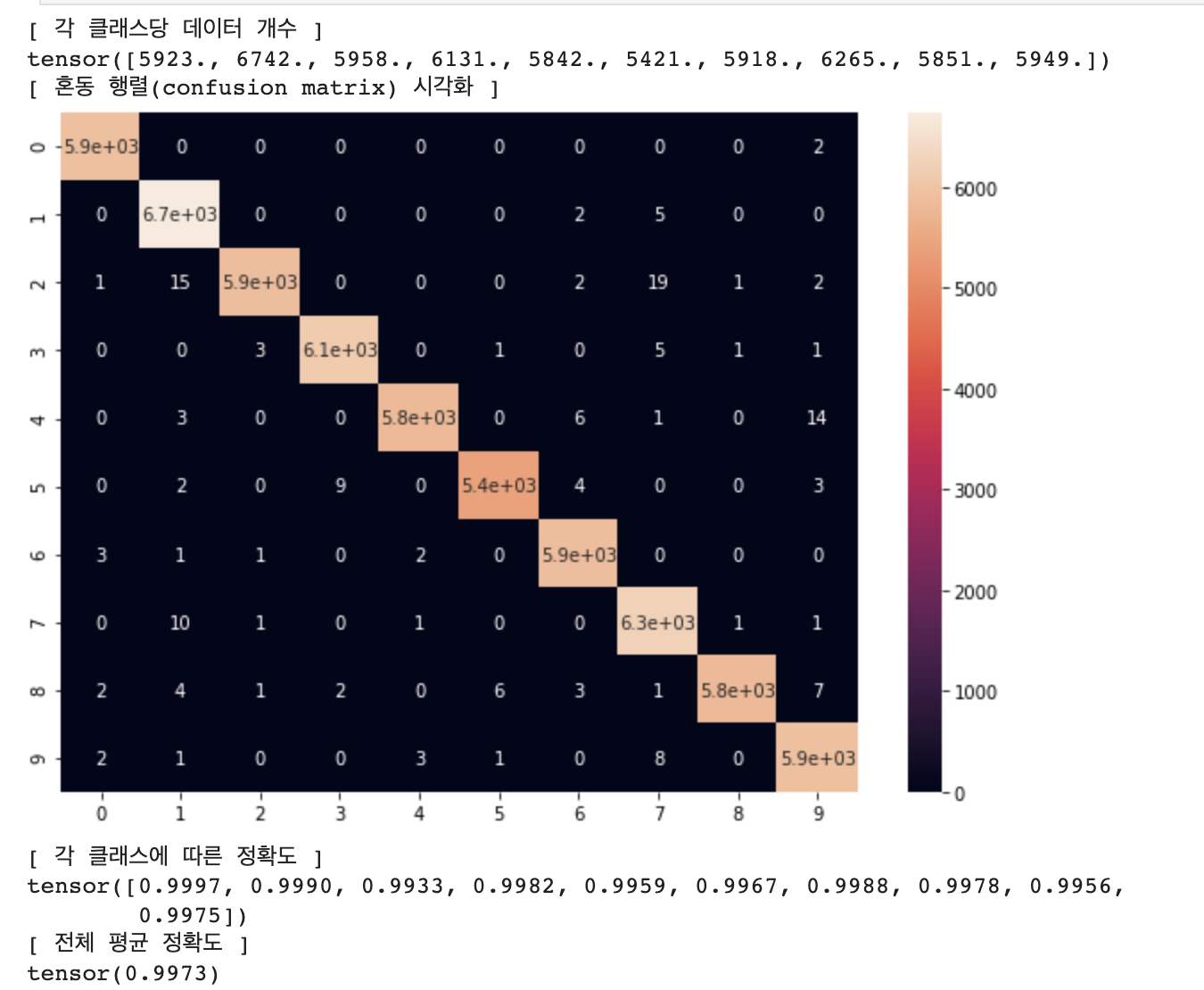
# 혼동 행렬(Confusion Matrix) 시각화 (테스트 데이터셋)
net = LeNet()
net = net.to(device)

file_name = "./checkpoint/LeNet_MNIST.pt"
checkpoint = torch.load(file_name)
net.load_state_dict(checkpoint['net'])

confusion_matrix = get_confusion_matrix(net, 10, test_loader)
print("[ 각 클래스당 데이터 개수 ]")
print(confusion_matrix.sum(1))

print("[ 혼동 행렬(confusion matrix) 시각화 ]")
# 행(row)은 실제 레이블, 열(column)은 모델이 분류한 레이블
res = pd.DataFrame(confusion_matrix.numpy(), index = [i for i in range(10)], columns = [i for i in range(10)])
plt.figure(figsize = (10, 7))
sn.heatmap(res, annot=True)
plt.show()

print("[ 각 클래스에 따른 정확도 ]")
# (각 클래스마다 정답 개수 / 각 클래스마다 데이터의 개수)
print(confusion_matrix.diag() / confusion_matrix.sum(1))

print("[ 전체 평균 정확도 ]")
print(confusion_matrix.diag().sum() / confusion_matrix.sum())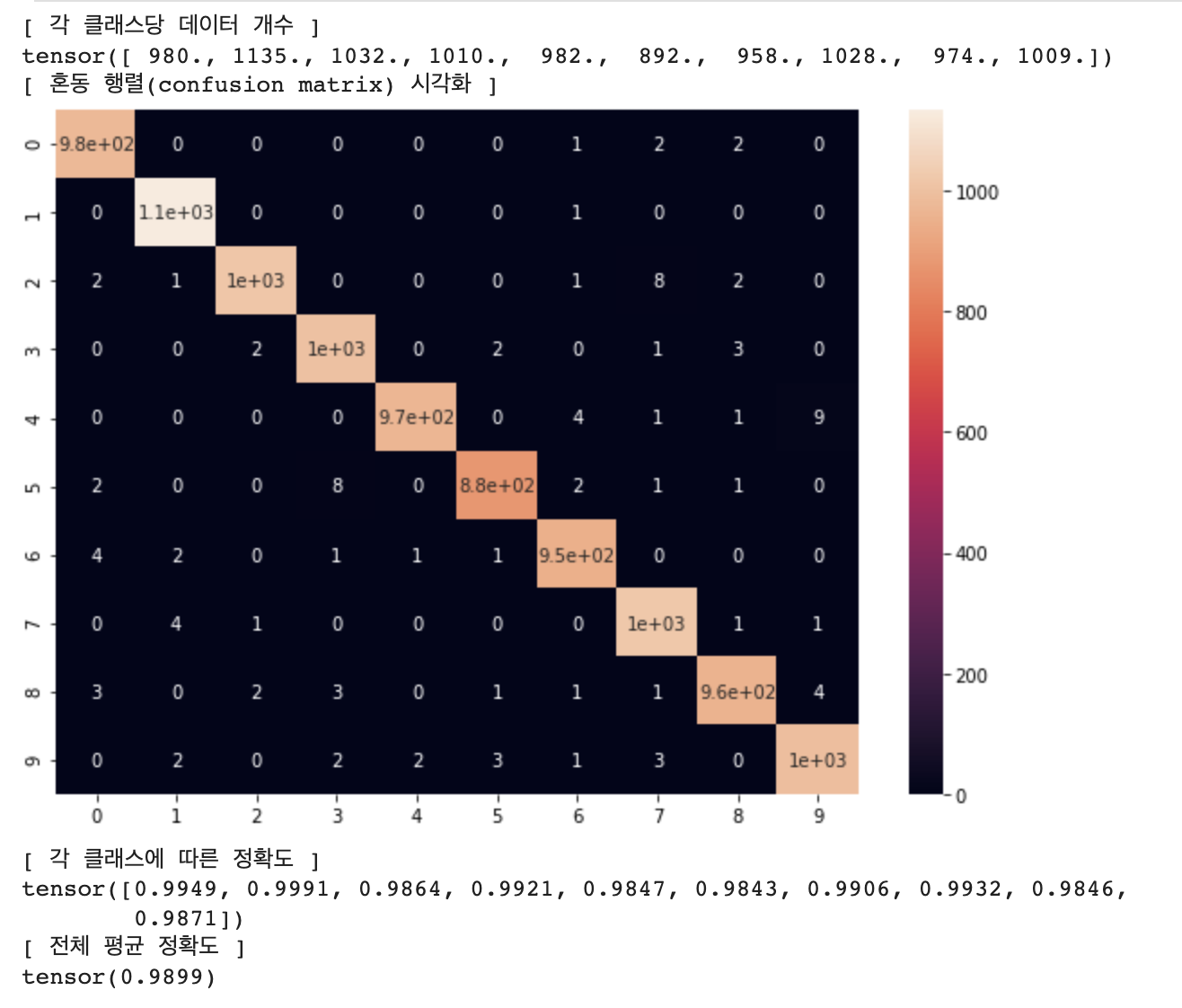
8. AlexNet 결과 분석
net = AlexNet()
net = net.to(device)

epoch = 10
learning_rate = 0.01
file_name = "AlexNet_MNIST.pt"

criterion = nn.CrossEntropyLoss()
optimizer = optim.SGD(net.parameters(), lr=learning_rate, momentum=0.9, weight_decay=0.0002)

train_result = []
test_result = []

train_result.append(evaluate(net, 0, file_name, train_loader, "Train"))
test_result.append(evaluate(net, 0, file_name, test_loader, "Test"))

for i in range(epoch):
    train(net, i, optimizer, criterion, train_loader)
    train_acc, train_loss = evaluate(net, i + 1, file_name, train_loader, "Train")
    test_acc, test_loss = evaluate(net, i + 1, file_name, test_loader, "Test")

    state = {
        'net': net.state_dict()
    }
    if not os.path.isdir('checkpoint'):
        os.mkdir('checkpoint')
    torch.save(state, './checkpoint/' + file_name)
    print('Model Saved!')

    train_result.append((train_acc, train_loss))
    test_result.append((test_acc, test_loss))
accuracy 커브 시각화
# 정확도(accuracy) 커브 시각화
plt.plot([i for i in range(epoch + 1)], [i[0] for i in train_result])
plt.plot([i for i in range(epoch + 1)], [i[0] for i in test_result])
plt.xlabel("Epoch")
plt.ylabel("Accuracy")
plt.legend(["train", "test"])
plt.show()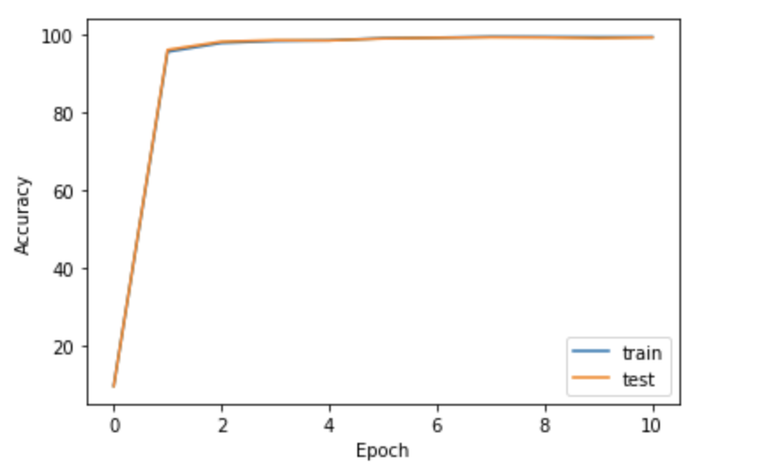
loss 커브 시각화
# 손실(loss) 커브 시각화
plt.plot([i for i in range(epoch + 1)], [i[1] for i in train_result])
plt.plot([i for i in range(epoch + 1)], [i[1] for i in test_result])
plt.xlabel("Epoch")
plt.ylabel("Loss")
plt.legend(["train", "test"])
plt.show()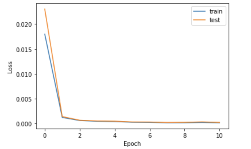
혼동 행렬(Confusion Matrix) 시각화 (학습 데이터셋)
# 혼동 행렬(Confusion Matrix) 시각화 (학습 데이터셋)
net = AlexNet()
net = net.to(device)

file_name = "./checkpoint/AlexNet_MNIST.pt"
checkpoint = torch.load(file_name)
net.load_state_dict(checkpoint['net'])

confusion_matrix = get_confusion_matrix(net, 10, train_loader)
print("[ 각 클래스당 데이터 개수 ]")
print(confusion_matrix.sum(1))

print("[ 혼동 행렬(confusion matrix) 시각화 ]")
# 행(row)은 실제 레이블, 열(column)은 모델이 분류한 레이블
res = pd.DataFrame(confusion_matrix.numpy(), index = [i for i in range(10)], columns = [i for i in range(10)])
plt.figure(figsize = (10, 7))
sn.heatmap(res, annot=True)
plt.show()

print("[ 각 클래스에 따른 정확도 ]")
# (각 클래스마다 정답 개수 / 각 클래스마다 데이터의 개수)
print(confusion_matrix.diag() / confusion_matrix.sum(1))

print("[ 전체 평균 정확도 ]")
print(confusion_matrix.diag().sum() / confusion_matrix.sum())
혼동 행렬(Confusion Matrix) 시각화 (테스트 데이터셋)
# 혼동 행렬(Confusion Matrix) 시각화 (테스트 데이터셋)
net = AlexNet()
net = net.to(device)

file_name = "./checkpoint/AlexNet_MNIST.pt"
checkpoint = torch.load(file_name)
net.load_state_dict(checkpoint['net'])

confusion_matrix = get_confusion_matrix(net, 10, test_loader)
print("[ 각 클래스당 데이터 개수 ]")
print(confusion_matrix.sum(1))

print("[ 혼동 행렬(confusion matrix) 시각화 ]")
# 행(row)은 실제 레이블, 열(column)은 모델이 분류한 레이블
res = pd.DataFrame(confusion_matrix.numpy(), index = [i for i in range(10)], columns = [i for i in range(10)])
plt.figure(figsize = (10, 7))
sn.heatmap(res, annot=True)
plt.show()

print("[ 각 클래스에 따른 정확도 ]")
# (각 클래스마다 정답 개수 / 각 클래스마다 데이터의 개수)
print(confusion_matrix.diag() / confusion_matrix.sum(1))

print("[ 전체 평균 정확도 ]")
print(confusion_matrix.diag().sum() / confusion_matrix.sum())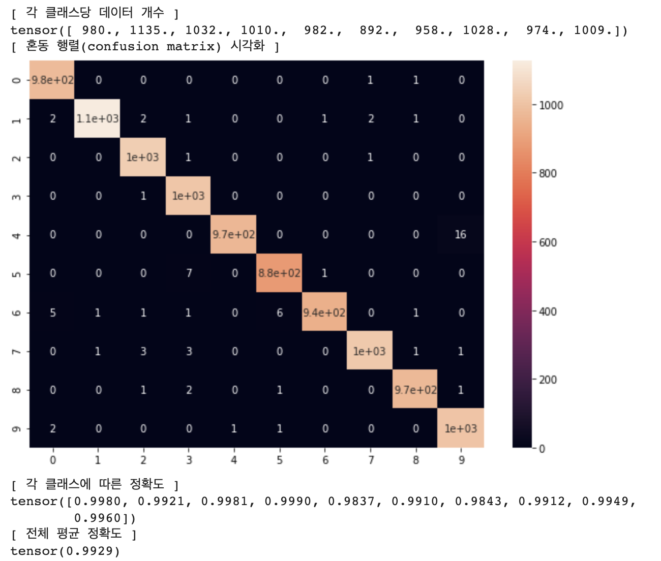
코드와 결과는 깃헙에 저장되어있습니다.
https://github.com/Kdavid2355/ai_code/blob/main/CNN_for_MNIST.ipynb
'인공지능공부' 카테고리의 다른 글
| ImageNet Pretrained ResNet 으로 MNIST 분류기 만들기 (0) | 2023.08.15 |
|---|---|
| DNN을 활용한 MNIST 분류 모델 구현 (0) | 2023.08.07 |
| [기계학습 입문] 타이타닉 생존자 예측 모델 Baseline 구축하기 (1) | 2023.07.23 |
| 다변수 선형회귀, Multivariable Linear Regression Pytorch 구현하기 (0) | 2023.07.23 |
| Linear Regression Pytorch 로 구현하기 (0) | 2023.07.23 |


