
| 일 | 월 | 화 | 수 | 목 | 금 | 토 |
|---|---|---|---|---|---|---|
| 1 | 2 | 3 | 4 | 5 | 6 | 7 |
| 8 | 9 | 10 | 11 | 12 | 13 | 14 |
| 15 | 16 | 17 | 18 | 19 | 20 | 21 |
| 22 | 23 | 24 | 25 | 26 | 27 | 28 |
| 29 | 30 |
- 플러터
- map
- 자연어처리
- AI
- Computer Vision
- 크롤링
- 42서울
- filtering
- RNN
- 유데미
- 선형회귀
- 앱개발
- CV
- 딥러닝
- 코딩애플
- 회귀
- 선형대수학
- pytorch
- 크롤러
- Flutter
- 인공지능
- 지정헌혈
- 42경산
- mnist
- 피플
- 파이썬
- 머신러닝
- Regression
- 모델
- 데이터분석
- Today
- Total
David의 개발 이야기!
[Pytorch] 파이토치 완전정복 part1 본문
< 머신러닝 시스템을 개발하는 것은 다음과 같은 과정을 따른다. >
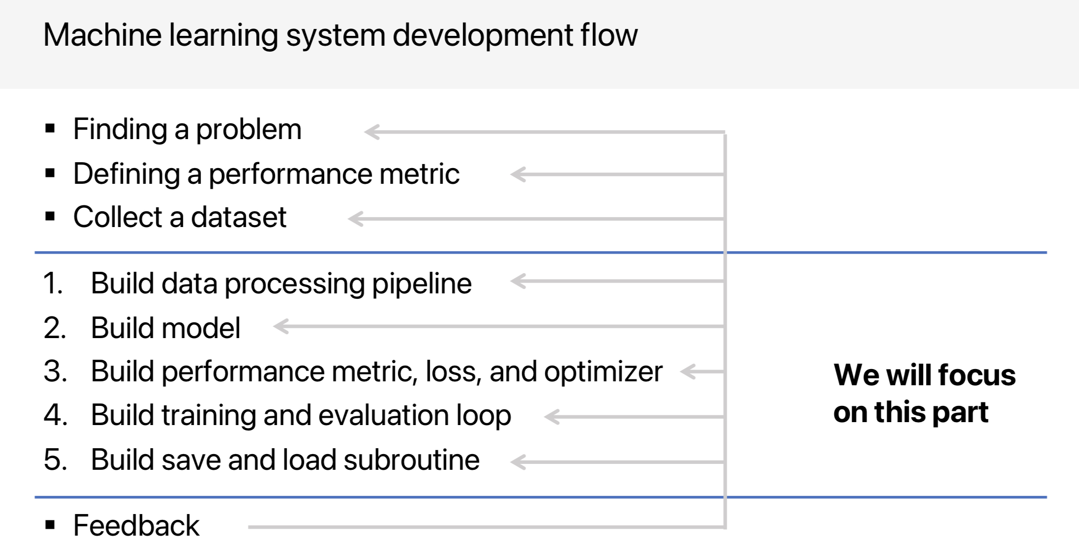
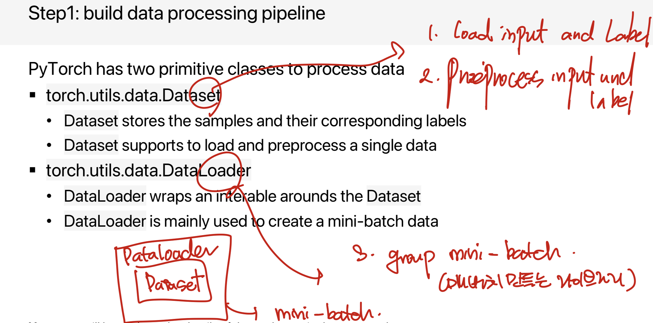
Step 1. Build data processing pipeline
대부분의 머신러닝 시스템은 모델을 학습시키기 위해 미니배치를 사용한다. 따라서, 금번 실습에서는 미니배치를 활용해 학습/평가를 진행하고자 한다. 세부 단계는 아래와 같다.
1. Load inputs and labels
2. Preprocess inputs and labels
3. Group inputs and labels as a mini-batch
Step 2. Build Model
인풋을 통해 예측 혹은 분류를 진행하는 모델을 정의한다.
1. Which model should be used?
2. How to set the hyperparameters of the model?
Step 3. Build performance metric, loss, and optimizer
P(W) == Performance of test set
L(W) == Maximizing performance on the test set by minimizing loss on the training set
Optimizer == SGD, Adam, AdamW...
Step 4. Build training and evaluation loop
training loop은 labels 과 predictions 사이의 loss를 계산하고자 함이다. 그리고, train dataset을 통해 model의 파라미터를 업데이트한다. evaluation loop은 validation set 또는 test set을 이용해서 성능을 평가하기 위함이다.
Step 5. Build save and load subroutine
Loading pre-trained parameters makes the trained model reusable
The training model is a very time-consuming process, save and load model parameters are essential subroutines in machine learning systems.
코드 구현하기
0. Import Pytorch Package
torch.nn : 모델 디자인
torch.optim : optimizer
Dataset , DataLoader : data processing을 위한 라이브러리
import os
import torch
import torch.nn as nn
import torch.optim as optim
import torchvision.transforms as T

from torch.utils.data import DataLoader
from torchvision.datasets import FashionMNIST
from torchmetrics import Accuarcy
from torchmetrics.aggregation import MeanMetric
1. Build Configuration
title = 'FashionMNIST'
device = 'cuda' if torch.cuda.is_available() else 'cpu'
data_root = 'data'
batch_size = 64
base_lr = 0.01
momentum = 0.9
epochs = 20
checkpoint_dir = 'checkpoint'
2. Build Data processing pipeline
train_transform = T.Compose([
	T.ToTensor(),
    T.Normalize((0.5, ), (0.5, )),
])
train_data = FashionMNIST(data_root, train=True, download=True, transform=train_transform)
train_loader = DataLoader(train_data, batch_size=batch_size, shuffle=True)

val_transform = T.Compose([
	T.ToTensor(),
    T.Normalize((0.5, ), (0.5, )),
])

val_data = FashionMNIST(data_root, train=False, download=True, transform=val_transform)
val_loader = DataLoader(val_data, batch_size=batch_size)
3. Build Model
To define a Model, we create a class that inherits from torch.nn.Module
The Module class has two important functions
- __init__ : Defines the layers of networks
- forward : Specifies how data will pass through the network
=> To accelerate opertaions in the neural network, we can move it to GPU if available, using function "to"
Class MyModel(nn.Module):
	def __init__(self):
    	super(MyModel, self).__init__()
        self.head = nn.Linear(28 * 28, 10)

    def forward(self, x):
    	x = x.reshape((x.shape[0], -1))
        x = self.head(x)
        return x

model = MyModel()

model = model.to(device)
텐서의 reshape 메소드는 텐서의 형태를 바꾸는데 사용된다.
-1은 PyTorch에게 해당 차원의 크기를 자동으로 계산하도록 요청하는 것이다.
CHATGPT 설명
우리가 28x28 크기의 이미지들로 이루어진 배치를 가지고 있습니다. 배치의 크기가 32라면, 이 데이터의 형태 (shape)는 [32, 28, 28]이 됩니다. 여기서 32는 배치의 크기, 28x28는 이미지의 높이와 너비입니다. 이제 이 데이터를 선형 레이어에 통과시키기 위해 이미지를 평평하게 만들어야 합니다. 이를 위해 각 이미지의 모든 픽셀을 연속된 배열로 만듭니다. 따라서 각 이미지는 길이가 28 * 28 = 784인 벡터가 됩니다. 그러면 데이터 전체의 형태는 [32, 784]가 됩니다
x.shape[0]는 배치의 크기, 즉 32입니다.-1은 해당 차원의 크기를 자동 계산하도록 PyTorch에게 요청하는 것입니다.
여기서는 784가 자동으로 계산되어 들어갑니다.
따라서 x.reshape((32, -1))의 결과는 [32, 784] 형태의 텐서가 됩니다.
4. Build Performance metric, loss, and optimizer
- To evaluate a model, we need a performance metric function.
- To train a model, we need loss function, an optimizer, and a learning rate scheduler
optimizer = optim.SGD(model.parameters(), lr=base_lr, momentum=momentum)

scheduler = optim.lr_scheduler.CosineAnnealingLR(optimizer, epochs * len(train_loader))

loss_fn == nn.CrossEntropyLoss()

metric_fn = Accuracy(task='multiclass', num_classes=10)
metric_fn = metric_fn.to(device)
4. Build training loop
In a training loop, the model makes predictions on the train set(fed to it in batches) and then backpropagates the predictions error to update its trainable parameters.
A training loop repeats the following steps:
1. Load a batch data from DataLoader
2. Froward propagation
3. Backward propagation
4 Update statistic
def train(loader, model, optimizer, scheduler, loss_fn. metric_fn, device):
	model.train()
    loss_mean = MeanMetric()
    metric_mean = MeanMetric()

    for inputs, targets in loader:
    	#device로 데이터 옮기기
        inputs = inputs.to(device)
        targets = targets.to(device)

        # Forward
        outputs = model(inputs)
        loss = loss_fn(outputs, targets)
        metric = metric_fn(outputs, targets)

        # Backward
        optimizer.zero_grad()
        loss.backward()
        optimizer.step()

         # Update statistics
        loss_mean.update(loss.to('cpu'))
        metric_mean.update(metric.to('cpu'))

        # Update learning rate
        scheduler.step()

    # Summarize statistics
    summary = {'loss': loss_mean.compute(), 'metric': metric_mean.compute()}

    return summary
5. Build evaluationing loop
In an evaluation loop, the model makes predictions on the validation or test set (fed to it in batches), and then backpropagates the prediction error to update its trainable parameters.
A Evaluation loop repeats the following steps:
1. Load a batch data from DataLoader
2. Forward propagation
3. Update statistic
def evaluate(loader, model, loss_fn, metric_fn. device):
	model.eval()
    loss_mean = MeanMetric()
    metric_mean = MeanMetric()

    for inputs, targets in loader:
    	inputs = inputs.to(device)
        targets = targets.tod(device)

        #Forward
        with torch.no_grad()
        	outputs = model(inputs)
        loss = loss_fn(outputs, targets)
        metric = metric_fn(outputs, targets)

        #Update statistics
        loss_mean.update(loss.to('cpu')
        metric_mean.update(metric.to('cpu')

    # Summarize statistics
    summary = {'loss': loss_mean.compute(), 'metric': metric_mean.compute()}

    return summary
6. Run training and evaluation loop + save model
The training process is conducted over several iterations (epochs). During each epoch, the model learns parameters to make better predictions. We print model's accuarcy and loss at each epoch. We would like to see the accuarcy increase and the loss decrease with every epoch.
for epoch in range(epochs):
    # train one epoch
    train_summary = train(train_loader, model, optimizer, scheduler, loss_fn, metric_fn, device)

    # evaluate one epoch
    val_summary = evaluate(val_loader, model, loss_fn, metric_fn, device)

    # print log
    print((f'Epoch {epoch+1}: '
           + f'Train Loss {train_summary["loss"]:.04f}, '
           + f'Train Accuracy {train_summary["metric"]:.04f}, '
           + f'Test Loss {val_summary["loss"]:.04f}, '
           + f'Test Accuracy {val_summary["metric"]:.04f}'))

    # save model
    state_dict = {
        'epoch': epoch + 1,
        'model': model.state_dict(),
        'optimizer': optimizer.state_dict(),
    }
    checkpoint_path = f'{checkpoint_dir}/{title}_last.pth'
    torch.save(state_dict, checkpoint_path)
7. Load Model and Comparison with randomly initialized model
# Load model
model_pretrained = MyModel()

checkpoint_path = f'{checkpoint_dir}/{title}_last.pth'
state_dict = torch.load(checkpoint_path)

model_pretrained.load_state_dict(state_dict['model'])

# Comparison with randomly initialized model
model_random = MyModel()

model_random.to(device)
model_pretrained.to(device)

random_summary = evaluate(val_loader, model_random, loss_fn, metric_fn, device)
pretraiend_summary = evaluate(val_loader, model_pretrained, loss_fn, metric_fn, device)

print(f'[Random] Test Acc {random_summary["metric"]:.04f}')
print(f'[Pretrained] Test Acc {pretraiend_summary["metric"]:.04f}')
여기까지가 기본적인 Pytorch 기본 코드이다.
이를 변형해서, 확장/발전 시켜나갈 수 있다.